Named Ranges with Column Headings

Let’s take the concept of named ranges a little further. Its true that the TABLE capabilities in later versions of excel give you much more opportunity to organize your data than before, but if we want many people to use our worksheets we cant rely on people have the latest versions.

Page Content hide

1 How to use Named with column headings.

2 Set up this date to follow along in a worksheet called ‘complicated sheetname’

3 Dynamic columns of data

4 Now we have everything defined – so what?

5 Why use named ranges with column headings

How to use Named with column headings.

By now you should be used to the idea of dynamic named ranges. You created a named range ‘MyExpenses’, using the definition

=OFFSET('complicated sheetname'!$A$2,0,0,COUNT('complicated sheetname'!$A$2:$A$10000),1)

Thats fine, but let’s say we want to use a complete set of related and then set up named ranges that are relative to wherever and whatever that set of data is, and lets say that new columns might be added, or the data rearranged, and you don’t want to have to go through the workbook fixing that every time it happens

Set up this date to follow along in a worksheet called ‘complicated sheetname’

We used this data on the right to introduce named ranges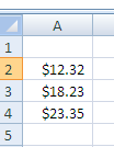

Let’s change that and add another column and some headings

You are first going to define a named range, MyExpensesBlock that will describe the whole block of data, including the titles

=OFFSET('complicated sheetname'!$A$1,0,0,COUNTA('complicated sheetname'!$A:$A),COUNTA('complicated sheetname'!$1:$1))

Lets break that down – will calculate the number of rows. Try it in an unused cell answer should be 4.

=COUNTA('complicated sheetname'!$A:$A)

.. and the number of columns. Try it in an unused cell answer should be 2.

=COUNTA('complicated sheetname'!$1:$1)

. once defined check the number of rows in your newly defined named range. Should be 4.

=ROWS(MyExpensesBlock)

.. and columns should be 2

=COLUMNS(MyExpensesBlock

Now, wherever you are in your workbook, you can just refer to ‘MyExpensesBlock’, and it will be the size and shape of the data in it. You can just forget all about the actual physical location as we go ahead and define named ranges for the individual data items.

Dynamic columns of data

As mentioned before, we want to protect the formulas in your workbook from any changes in size,location and structure that happen in MyExpensesBlock

We are going to define three more named ranges – MyExpensesHeadings, MyExpenses, and MyExpensesItems, which are the item names in row 1, the amounts in Column B, and the Items in column A – but we are going to do that without mentioning columns, rows or worksheet references.

Define MyExpensesHeadings as below, which means 1 row deep, 0 columns and 0 rows away from the beginning of myexpensesBlock. Test ROWS(myExpensesHeadings) & COLUMNS(myExpensesHeadings). The answers should be 1 and 2.

=OFFSET(myExpensesBlock ,0,0,1)

Define MyExpenses as below

=OFFSET(myExpensesBlock ,1,MATCH("Expenses",myExpensesHeadings,0)-1,rows(myexpensesb

Let’s break that down – Find the column titled ‘Expenses’. Match returns a value 1-n, so we need to subtract 1 for use by offset, which starts counting from 0. Try in an unused cell. Answer should be 1

=MATCH("Expenses",myExpensesHeadings,0)-1

…the number of data rows would be the number of rows in the data block -1 for the header. Should be 3

=rows(myexpensesblock)-1

Putting it all together it would translate as this – 3 rows of data, 1 column to the right, and one column down from the beginning of myExpensesBlock

=OFFSET(myExpensesBlock ,1,1 ,3,1)

.. once defined check the number of rows in your newly defined named range. Should be 3

=ROWS(MyExpenses)

.. and columns should be 1

=COLUMNS(MyExpenses)

Define MyExpensesItems as below, and repeat the tests above, substituting myExpensesItems for MyExpenses. Note the only difference between the two definitions is the heading title – “Items” instead of “Expenses”. You can see that it would be very easy to set up many columns of data like this, and since everything is derived from other dynamic named ranges, the only time you have to refer to actual cell references is in the initial definition of the Block of data.

=OFFSET(myExpensesBlock ,1,MATCH("Items",myExpensesHeadings,0)-1,rows(myexpensesblock)-1,1)

Now we have everything defined – so what?

Well now we can start using these throughout the workbook. But you can really start to see the coolness of all this if you start to modify your datablock. Set up the formulas below in some unused cells. Try swapping the Items & Expenses Columns. Add extra columns. Add extra Rows. For as long as you don’t change the column titles, everything will still work.

Now that you have verified that all this is working, goto another sheet and enter. The result should be $53.90

=SUM(MyExpenses)

Now that you have verified that all this is working, goto another sheet and enter. The result should be 3

=COUNTA(MyExpensesItems)

You can use negative offsets too. This should give you “Items”.

=Offset(MyExpensesItems,-1,0,1,1)

Why use named ranges with column headings

In a word Flexibility. As you bring in additional rows and columns of data, everything will still work and you shouldn’t have to change any formulas which reference these ranges.

For help and more information join our forum, follow the blog or follow me on Twitter