Search() and Find() are pretty much the same. The only difference is that Find worries about matching case (upper/lower) and search doesn’t. That means that Brass is the same as brass as far as Search is concerned, but find thinks they are different. So you can equally apply everything I say about search here to find. SEARCH() is a function that can very quickly turn into something very complex if you are using it, for example, to split up a list a,b,c,d… into separate cells. This is a common thing to want to do, and I don’t understand why there is not a simplified way to do this. It is easy enough in VBA of course, but the majority of Excel users want to do things right there, by means of a built in function. In any case the fact that SEARCH() enables this kind of complex string manipulation makes for a good learning exercise.
What is Search()
Here is the definition, pretty straightforward – but we’ll see how to use it in an odd way later…
In Excel, the Search function returns the location of a sub-string in a string. The search is NOT case-sensitive.
The syntax for the Search function is:
Search( text1, text2, start_position )
text1 is the substring to search for in text2.
text2 is the string to search.
start_position is the position in text2 where the search will start. The first position is 1.
If the Search function does not find a match, it will return a #VALUE! error.
An example of where you could use it
First create a new sheet called Uses, and enter this
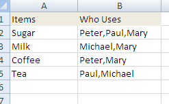
We are going to check whether Paul uses Sugar. Very easy since SEARCH() will return a number or not.
=IF(ISNUMBER(SEARCH(“Paul”,B2)),”Paul Uses Sugar”,”Paul doesn’t Use Sugar”)
Lets expand that a bit, and change your Uses sheet to look like this – leave cells c2:I5 blank for now. We are going to fill them in with various formulas as we go through these examples.
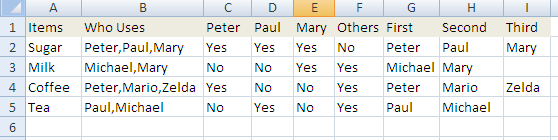
Now C2:E5 look pretty straightforwards – put this formula in C2 and fill over and down – nothing new there.
=IF(ISNUMBER(SEARCH(C$1,$B2)),”Yes”,”No”)
But how about F2:F4 ? Here we are looking for people mentioned in column B who are not Peter,Paul or Mary. Actually we are not going to use SEARCH() for that. We are going to count the commas and compare that against the number of times we’ve seen Yes in columns C through E. Counting the commas is actually pretty easy. Use SUBSTITUTE() to get rid of the commas then subtract the number of characters before and after. The answer is the number of commas. I’ve added 1 for the comma that should be at the end of B2. Strictly speaking I should have tested to see if there was one there already, and I should also have tested for B2 being blank – but you get the idea anyway I think.
=IF(LEN(B2)-LEN(SUBSTITUTE(B2,”,”,””))+1- COUNTIF(C2:E2,”Yes”)>0,”Yes”,”No”)
Using Nested Search()
Now we get to the interesting part. How to split “Who Uses”, into First, Second and Third mentioned. To do this we are going to use MID() and SEARCH(). It gets complicated really quickly so you have to be careful to put brackets commas etc in the right place. Column G, the first one is easy. I’ve added IFERROR() just to avoid getting the #VALUE error if there is nobody. You can omit that if you want. It was an Excel 2007 addition. I’ve also added a comma to the end of B2. Again I should have tested to see if it was already there etc. as per my previous comments. Essentially this is just taking the 1st part of the string up to the first comma. Put this in G2 and fill down.
=IFERROR(MID(B2,1,SEARCH(“,”,B2 & “,”)-1),””)
Column H, the second one is more complicated. In this case we have to take the part of the string after the first comma, but before the second. SEARCH() has an optional 3rd argument Search( text1, text2, start_position ) and we are going to need to use that start_position to indicate where the first comma occurred. Put this is H2 and fill down.
=IFERROR(MID(B2,SEARCH(",",B2 & ",")+1,SEARCH(",",B2 & ",",SEARCH(",",B2 & ",")+1)-SEARCH(",",B2 & ",")-1),"") Lets break that down. The first occurrence is going to tell us where the 1st character after the first comma is, so MID() can use that to know where the extraction has to startSEARCH(",",B2 & ",")+1
but what about the length? Well, you have to know where the 2nd comma is for that, so we have to use a nested SEARCH(). That means that we use the position of the 1st comma + 1 as the optional start_position argument to find the 2nd comma. Finally we need to subtract the length of the string that took us up to the 1st commaSEARCH(",",B2 & ",",SEARCH(",",B2 & ",")+1)-SEARCH(",",B2 & ",")-1)
Column I, Things start to get unreadable. However the principle is very easy and exactly the same as Column H. This time we need to find whats between the 2nd and third comma, so we continue to build up the nesting of SEARCH() to include everything thats gone before. Put this in column I and fill down.
=IFERROR(MID(B2,SEARCH(",",B2 & ",",SEARCH(",",B2 & ",")+1)+1,SEARCH(",",B2 & ",",SEARCH(",",B2 & ",",SEARCH(",",B2 & ",",SEARCH(",",B2 & ",")+1)+1)-SEARCH(",",B2 & ",")+1)-1),"")
Preparing this data for future use elsewhere
We may use some of this data in further examples, so you can go ahead and set up the named ranges for them now so we wont have to worry about where it is later. create MyUsesBlock, MyUsesHeadings, MyUsesItems, MyUsesWho according to the method in Named Ranges with Column Headings. You should end up with the following definitions MyUsesBlock
=OFFSET(‘Uses’!$A$1,0,0,COUNTA(‘Uses’!$A:$A),COUNTA(‘Uses’!$1:$1))
MyUsesHeadings
=OFFSET(myUsesBlock ,0,0,1)
MyUsesItems
=OFFSET(myUsesBlock ,1,MATCH(“Items”,myUsesHeadings,0)-1,rows(myUsesblock)-1,1)
MyUsesWho
=OFFSET(myUsesBlock ,1,MATCH(“Who Uses”,myUsesHeadings,0)-1,rows(myUsesblock)-1,1)
Sorting chapter/bullets numbers
Quite often you need to sort data that has some kind of chapter numbering, such as
1.1
1.1.2
2.1.1
2.12.2
A specialized form of this would be ip numbers, for example
192.1.3.2
172.12.180.1
These do not lend themselves to sorting easily, so the obvious solution is to insert leading zeroes. The problem though is how to separate the individual components so as to be able to standardize their widths.
One way is to use the search function in Excel. Here is an example of turning such a form into a set of 4 digit numbers so they can be sorted (1.12.11 into 0001.0012.0011.). Let’s say that the input 1.12.11 is in cell B15, the formula is very complex, and becomes exponentially more complex with more groups of numbers.
=TEXT(IFERROR(MID(B15,1,SEARCH(“.”,B15&”,”)-1),””),REPT(“0″,4)&”.”) & TEXT(IFERROR(MID(B15,SEARCH(“.”,B15 & “.”)+1,SEARCH(“.”,B15 & “.”,SEARCH(“.”,B15 & “.”)+1)-SEARCH(“.”,B15 & “.”)-1),””),REPT(“0″,4)&”.”)& TEXT(IFERROR(MID(B15,SEARCH(“.”,B15 & “.”,SEARCH(“.”,B15 & “.”)+1)+1,SEARCH(“.”,B15 & “.”,SEARCH(“.”,B15 & “.”,SEARCH(“.”,B15 & “.”,SEARCH(“.”,B15 & “.”)+1)+1)-SEARCH(“.”,B15 & “.”)+1)-1),””),REPT(“0″,4)&”.”)
A better way is to use a regEx approach. Although regEx is available in VBA, it is not directly usable as a spreadsheet function. The Excel RegEx library allows you to use a prebuilt library of regexes or to use your own directly in your spreadsheet. Here is the solution to the same problem using regEx. Let’s say the regEx expression ([0-9]+).([0-9]+).([0-9]+) is in A15, and the value to be processed is in B15. The solution is
=TEXT(rxreplace(A15,B15,”$1″),REPT(“0″,4)&”.”) & TEXT(rxreplace(A15,B15,”$2″),REPT(“0″,4)&”.”) & TEXT(rxreplace(A15,B15,”$3″),REPT(“0″,4)&”.”)
In addition to being simpler to start with, complexity increase is linear as more sets of numbers are added.
Why use Search()
Search has a number of uses, in particular where the data came from some other source and you didn’t have the chance to organize it. Excel works best when all the data elements are in separate cells. Having multiple information in one cell never works very well. Search can help you split up the data into something more usable. The problem with search is that your formula can become complex, unwieldy and incomprehensible very quickly, especially if you have to nest, which is very often the case. Dealing with #VALUE errors is also tedious, especially pre- 2007 where you had to use IF(iserror(),,) rather than IFERROR(,,) You can simplify the above, by using helper cells which allow you to split the problem into more manageable chunks.