As I’ve said before you can use Sumproduct() for many things that it probably wasnt designed for. Various array functions could be used to do the same thing, but trying to do it all in sumproduct is more interesting
Prioritizing Lookups.
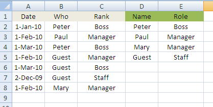
Lets say that we have a scenario where we have a signing in book which shows dates and people. There could be multiple people signing in on the same date. Each of these people has a role – lets say Boss, Manager and Staff, and we want to record against each entry whether there were any staff present on a day when no managers were..
Create a new sheet called guests with this information. You can leave column C blank for now, because our exercise is to create the formulas for C. You can see that we have identified row 7 as an example of a day when there were staff with no manager present.
Named ranges
Normally at this point we would create named ranges for all this data, but I’m going to use this example for illustration only and not use the elsewhere, so for now lets just stick to column references.
Approach
This is a tough one. We obviously can use use VLOOKUP() to translate Who into Rank.So lets do that right away to start. Put this is C2 and fill it down.
=VLOOKUP(B2,$D$2:$E$5,2,FALSE)
That does some of what we want, but we want C5 and C6 to say Manager (Paul was also present on 1st Feb) and Boss (Peter was present on 1st March)
So this is a tough nut to crack without some lateral thinking. Thats where SUMPRODUCT() comes in.
First lets identify the rows which don’t need to be modified. Essentially thats all those where there is not “Guest” in Column B..
=IF(B2<>"Guest",VLOOKUP(B2,$D$2:$E$5,2,FALSE), "What shall we do about these")
That gives us this
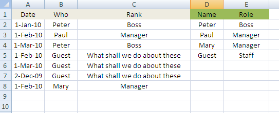
What we want to happen is that C7 looks up Staff, C5 looks up Manager, C6 looks up Boss.
Here is the formula. Put it in B2 and fill down.
=IF(B2<>"Guest",VLOOKUP(B2,$D$2:$E$5,2,FALSE), VLOOKUP(INDEX($B$1:$B$8, SUMPRODUCT( LARGE(--($A$2:$A$8=A2)* --($B$2:$B$8<>"Guest" )*ROW($B$2:$B$8),1))) ,$D$2:$E$5,2,FALSE))
Lets Break it down – we’ve already covered the 1st part, so lets focus on the 2nd part.
=VLOOKUP(INDEX($B$1:$B$8,SUMPRODUCT(LARGE(--($A$2:$A$8=A2)*--($B$2:$B$8<>"Guest" )*ROW($B$2:$B$8),1))),$D$2:$E$5,2,FALSE)
First the SUMPRODUCT() part.
=SUMPRODUCT(LARGE(--($A$2:$A$8=A2)*--($B$2:$B$8<>"Guest" )*ROW($B$2:$B$8),1))
One of the properties we discussed earlier about SUMPRODUCT() is that it actually produces an array result then adds up the items in the arrray. The trick here is to intercept the intermediate array result and pick something other than the current row that has the same date as the current row. How? Consider the intermediate stage in the formula above for Row 6.
=LARGE({0;0;1;0;1;0;0}*{1;1;1;0;0;0;1},*{2;3;4;5;6;7},1)
These are the rows where the date matches row 6, and these are the rows that are okay to use because they dont have Guest in them. Mutiplying those by the row number on which to find them will give the row numbers of every item that does not contain guest, and is on the same date as the current row. Finally we’ll pick the one with the highest row number, in case there were more than one candidate for the same day by using the LARGE() function. The result then of all that is 4. Which tells us to use Row 4 as the lookup source value rather than Row 6.
This takes us back to this simple operation to lookup with Row 4, Peter, rather than Row 6 Guest – exactly what we want.
=VLOOKUP(INDEX($B$1:$B$8,4),$D$2:$E$5,2,FALSE)
I think you would agree that this shows how SUMPRODUCT() can contribute towards many problems in unexpected ways. Watch this space for more.